ConceptTime: Predictive Surprise as Self-Grounding Concept Bottleneck for Interpretable Time Series

Interactive sketch on a synthetic signal using simplified versions of each stage. It shows the mechanism, not the paper's experiments. Click a step, or switch to “Unfamiliar input” to see abstention.

TL;DR. One frozen forecaster's surprise does three jobs at once: it decides where segments start and end, describes how each segment behaved, and tells the classifier when an input is outside what it knows. The result is an interpretable time-series classifier that needs no concept annotations, stays competitive with black-box models, and keeps near-98% accuracy on Epilepsy with just 1% of the labels.

17

public benchmarks across wearables, EEG, UEA, and fault diagnosis

97.91%

Epilepsy accuracy with only 1% of training labels

0.992

OOD AUROC of the built-in fidelity score (HAR, strongest noise)

94.37%

mean cross-domain transfer accuracy with 5% target labels

Abstract

Time-series classifiers deployed in risk-sensitive domains must be (1) accurate, (2) interpretable, and (3) able to abstain when evidence is weak. Existing methods do not deliver all 3 at once, and the obstacle is structural, rather than logistical. Meaningful temporal patterns cannot be defined without knowing segment boundaries, yet meaningful boundaries cannot be placed without knowing which patterns to expect. Existing approaches break this circularity by using fixed windows or expert-annotated vocabularies, thereby sacrificing at least one of the 3 properties.

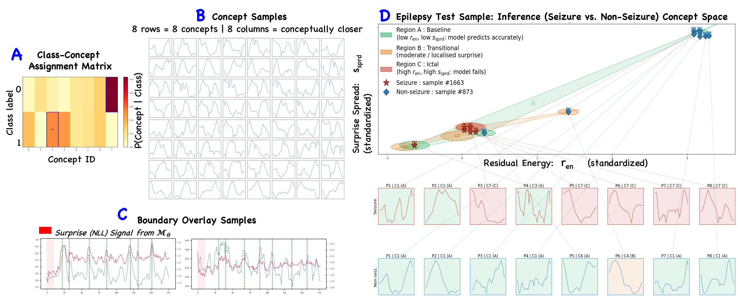
We introduce ConceptTime, which closes the loop through a single self-supervised signal. A frozen probabilistic forecaster predicts a distribution over the next observation at every timestep of the sequence. We call the mismatch between its prediction and the realized signal the predictive surprise. This signal both locates segment boundaries and characterizes each resulting segment through the forecaster. Segments are thus grounded by how they behaved relative to expectation, not by what they look like. These summaries cluster into a vocabulary of dynamical regimes that we call concepts. A lightweight head classifies from the concept sequence, and the distance to the nearest concept yields reliability by design.

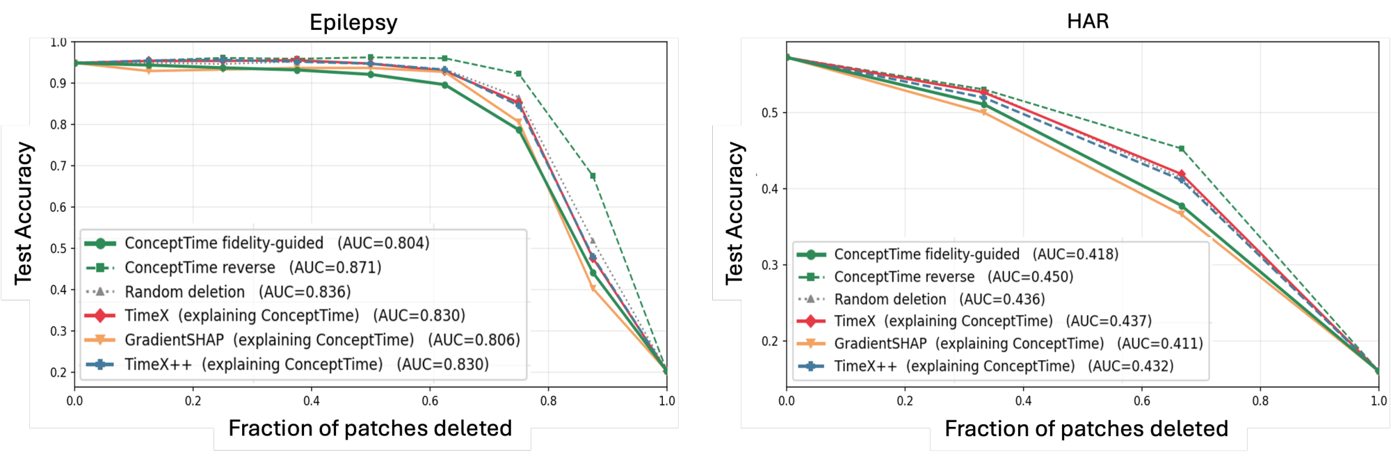
Across 17 public benchmarks, ConceptTime is competitive with state-of-the-art black-box accuracy, beats every interpretable baseline, and retains near-98% accuracy on Epilepsy with 1% of labels. It further remains competitive with softmax, prototype-distance, and SHAP/TimeX/TimeX++ on OOD detection and deletion faithfulness, without human annotations, language model calls, or domain experts.

The chicken-and-egg problem

Good concepts need good segment boundaries, and good boundaries need to know which concepts to look for.

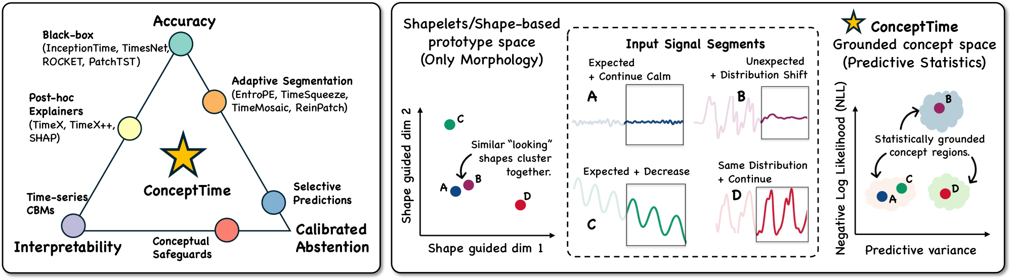
Prior concept-bottleneck methods for time series break this loop by splitting it into two stages: fixed windows or change-point thresholds first, concepts second. Each choice gives something up. Fixed-window models need predefined vocabularies and lose calibrated abstention. Adaptive-patching models segment well but expose no concepts. Vector-quantized tokens are discrete but carry no inherent meaning.

ConceptTime's observation is that the same signal that finds a boundary can also describe the segment. Two segments can look alike yet behave very differently given what came before them. Grouping segments by how they deviated from prediction, rather than by raw shape, separates dynamical regimes that shape-based vocabularies merge.

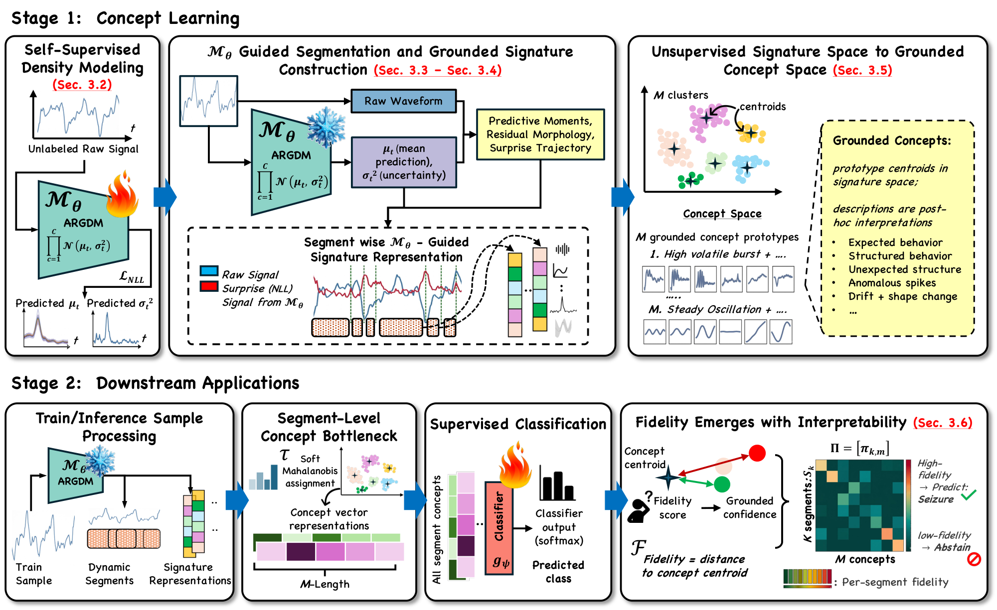
Left: a triangle of accuracy, interpretability, and calibrated abstention, with ConceptTime at the centre. Right: four segments A to D shown in a shape-based space and in a predictive-geometry space spanned by predictive variance and NLL. — **Figure 1.** Left: existing methods favour different goals. Right: raw-shape space merges segments A and B (both end calm) and separates C from D. Predictive-geometry space groups A, C, and D, where expectations were met, and isolates B as a surprise.

Method

Two stages with separate training signals. Labels touch only the final lightweight classifier.

1

Self-supervised density model

A 4-layer causal Transformer (ARGDM) predicts a diagonal Gaussian over the next step. A calibration regularizer keeps σ² honest. It is trained once, then frozen.

2

Surprise-guided segmentation

Per-step surprise s_t (NLL) drives length-constrained dynamic programming that places exactly K patches in O(TK), avoiding degenerate or collapsed segmentations.

3

Predictive-geometry concepts

Each patch gets a 2C+13-dimensional signature from predictive moments, residual morphology, and surprise trajectory. A GMM over signatures forms the concept vocabulary, with no labels and no concept leakage.

4

Classifier and fidelity

A small head (about 10³–10⁴ parameters) classifies the K×M concept tensor. Prototype distances give a fidelity score F(x) = exp(−Σ d_j / Kτ) for abstention at no extra cost.

Overview diagram of ConceptTime. Stage 1, concept learning: self-supervised density modelling, surprise-guided segmentation and signature construction, and clustering into grounded concept prototypes. Stage 2, downstream: segment-level concept bottleneck, supervised classification, and fidelity-based abstention. — **Figure 2.** Overview of ConceptTime. Stage 1 learns concepts from unlabeled signals; textual concept descriptions are post hoc, not training signals. Stage 2 maps new inputs to concepts by nearest-prototype assignment, classifies through the concept tensor, and uses each segment's prototype distance for abstention.

Results

Accuracy, label efficiency, transfer, and abstention, all from the same concept space.

Epilepsy accuracy, 1% labels

Accuracy (%). With few labels, ConceptTime beats every black-box baseline.

ConceptTime97.91
TSLANet95.41
InceptionTime95.14
MiniRocket94.71
TimesNet93.74
ROCKET93.68
TOTEM91.65
catch2286.03
VQShape81.00
ProSeNet65.51

Above the dashed line: black-box models. Below: interpretable baselines.

Cross-domain transfer

Mean target accuracy (%) over all 12 fault-diagnosis operating-condition pairs.

Target-M_θ, 5%94.37
Source-M_θ, 5%91.09
TSLANet, 5%90.76
Direct, 0%67.61

Highlighted rows are ConceptTime settings. The source concept vocabulary stays fixed; only the small classifier (and optionally the density model) adapts. Target-M_θ ranks first on 7 of 12 directions.

Out-of-distribution detection

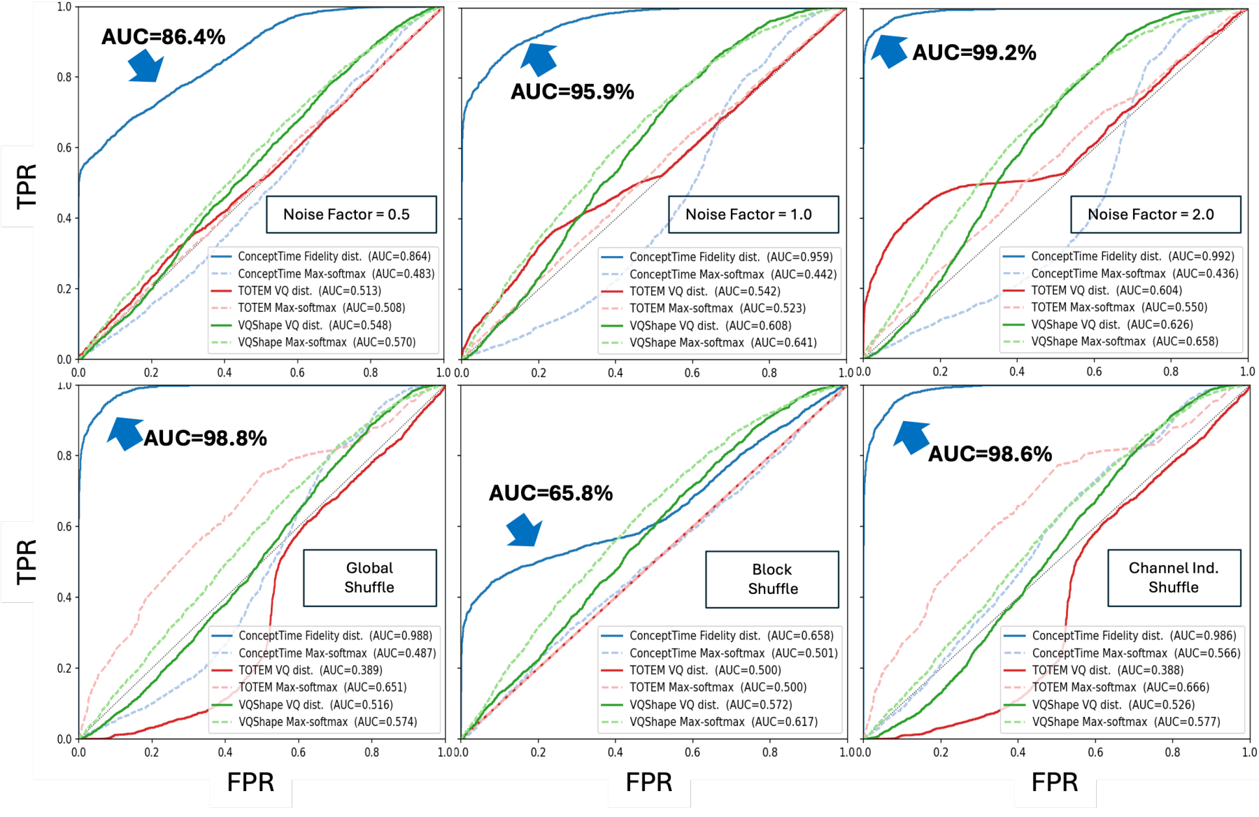
AUROC on HAR with Gaussian noise (factor 2.0). 0.5 is chance.

CT fidelity0.992
VQShape softmax0.658
VQShape VQ dist.0.626
TOTEM VQ dist.0.604
TOTEM softmax0.550
CT softmax0.436

Fidelity rises with shift severity (0.864 → 0.959 → 0.992 as the noise factor goes 0.5 → 2.0); the classifier's own softmax stays near chance.

+45.0 pts

Predictive geometry, not adaptive patching alone, drives the gain. On UCI-HAR, with the same adaptive patches and vocabulary size, predictive-moment signatures reach 87.7% accuracy versus 42.7% for raw-signal morphology. At full supervision ConceptTime matches black-box models on Epilepsy and trails them by 2–8 points elsewhere, the cost of enforcing a concept bottleneck.

Qualitative analysis on Epilepsy: class-concept assignment matrix, nearest patches per concept, surprise signal with segment boundaries, and seizure versus non-seizure segments in a residual-energy and surprise-spread concept space. — **Figure 5.** What the concepts look like on Epilepsy. (A) Although learned without labels, P(concept | class) peaks at different concepts for seizure and non-seizure. (B) Nearest patches to each prototype. (C) Boundaries coincide with surprise peaks. (D) Most seizure patches fall where the density model predicts poorly (region C); most non-seizure patches fall where it predicts well (region A).

ROC curves for OOD detection on HAR under three Gaussian-noise levels and three shuffle perturbations, comparing ConceptTime fidelity with softmax and prototype-distance scores. — **Figure 3.** OOD detection on HAR under Gaussian-noise and temporal-shuffle perturbations.

Deletion curves on Epilepsy and HAR comparing fidelity-ranked patch deletion with GradientSHAP, TimeX, TimeX++, random, and reverse orderings. — **Figure 4.** Deletion faithfulness (lower AUC is better). Fidelity gives the lowest AUC on Epilepsy (0.804); GradientSHAP leads narrowly on HAR (0.411 vs 0.418).

Limitations and future work

Fixed vocabulary sizeM is chosen in advance. Hierarchical vocabularies could capture patterns at several levels of detail.
Post-hoc meaningWhat each prototype means is decided by a person after training. Concept names are interpretations, not supervision.
Static conceptsOnline vocabulary updates could let concepts adapt as signal patterns drift over time.
Beyond classificationLow-fidelity segments could guide active relabeling, regime discovery, and anomaly localisation.

BibTeX

@inproceedings{abeywickrama2026concepttime,
  title     = {Predictive Surprise as Self-Grounding Concept Bottleneck
               for Interpretable Time Series},
  author    = {Abeywickrama, Sachith and Eldele, Emadeldeen and Wu, Min
               and Li, Xiaoli and Yuen, Chau},
  booktitle = {Advances in Neural Information Processing Systems (NeurIPS)},
  year      = {2026}
}